Should We Mind the ‘Reality Gap’?

It’s generally accepted that making education ‘relevant’ is a good thing for the classroom.  Usually, this means finding practical applications for theory.  But how much of a problem is it when our ‘real world’ examples aren’t as ‘real’ as they might appear?  How important is the ‘Reality Gap’?

A universal complaint of students, whether at school, college or university, is that they often don’t see the relevance of some of the material they study.  “When am I going to be doing this in a real job?” is a typical question.  There are three broad categories of response from the teacher; bluntly and clumsily characterised as follows:

1. “You’re getting an education that shows your capability at this level.  The content doesn’t matter.  You’ll be trained to do a particular job when you’ve got one.”
2. “You might only use about 10% of what you’re learning now in the real world but you don’t know which 10% it’s going to be and your 10% will be different to everyone else’s 10% so we have to do all this stuff.”
3. “Well, here’s an example of how this might be used in the real world.”

(A good teacher would add a considerable degree of finesse to these answers, of course.)  Ignoring the merits and demerits of 1 and 2 entirely, how best to achieve 3 presents some interesting challenges because, much as we might like to pretend otherwise, the real world is a terribly complicated place, in which the textbook usually only gets us so far …

Ben Goldacre’s well-made point about the limitations of political soundbites has wider applications.  On the whole, the real world ‘is a lot more complicated that that‘.  If we’re honest, just about nothing works in the real-world quite the way it does in the textbook.  There’s always a tweak, some missing data, a bit of pre-processing or some other extra step or a layer of subtlety that’s needed to make something work in practice – and sometimes things just don’t work at all.  A full menu would be all but endless but here are some diverse tasters:

• In the real world, robots don’t just ‘turn left’; they ‘turn on the left motor’ ‘until facing left’; then it’s a question of how to work that out in practice.  Similarly, a washing machine doesn’t just ‘fill with water’; it opens an inlet valve, keeps testing water level, etc.
• Cover and seal a burning candle and some water with a glass jar.  The water level rises by a fifth to replace the oxygen that’s burnt (20% of the air).  No, it’s more complicated than that.
• The perfect angle at which to fire a projectile to maximise the distance it travels is half-way between the angle of the plane it’s on and the vertical … unless you feel the need to take air resistance into account, that is.
• Internet routing protocols generally work by solving some form of graph optimisation problem.  This, in turn, involves minimising some ‘cost function’.  Unfortunately, what cost actually means in the Internet at large is anyone’s guess.  (We’ll come back to this one.)

Well, let’s pick an example to look at in a bit more detail and, presumably, it better be something in the Computer Science line.  Here’s another example of a graph optimisation problem and an algorithmic solution …

A Minimum Spanning Tree (MST) of a graph is a subset of the graph’s edges that completely connect the graph’s vertices at minimum cost.  Here’s an example of a graph and its MST:

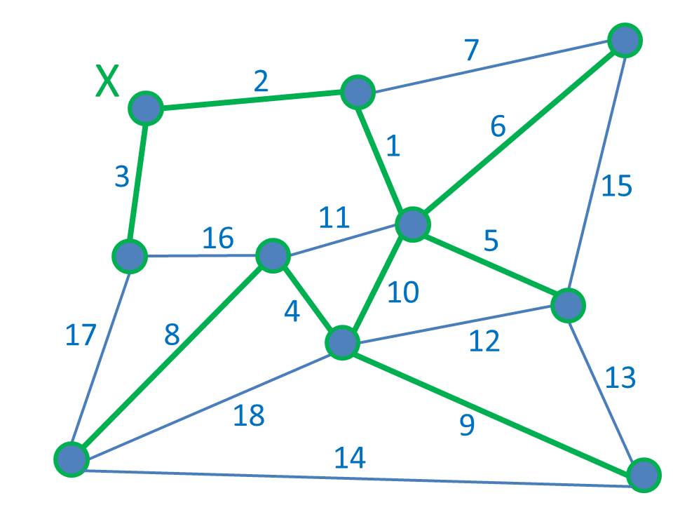
Imagine everything in the original graph starts off blue.  The numbers on each edge are the ‘costs’.  Here, for simplicity, the eighteen edges are labelled with costs running consecutively from 1 to 18 (but it doesn’t have to be like that).  The edges shown in green make up the MST, the least cost way of connecting all the vertices together.  Nice.

Mathematicians, Graph Theorists and Computer Scientists alike tend to like an MST because, not only is it an easy to define problem and an easy to understand solution, there’s even a simple algorithm to produce it – in fact there are two.

Kruskal’s Algorithm simply adds least cost edges anywhere in the graph, in increasing order, with the simple constraint that no added edge creates a loop with those (green) edges already there.  (A tree has no loops.)  Prim’s Algorithm, on the other hand, starts from one specific green vertex and, at each iteration, adds the cheapest edge connecting the green part of the graph to the blue part (thus spreading the green part).  So, for our example, Kruskal would add edges 1, 2, 3, 4, 5 & 6 before considering edge 7.  This would create a loop with edges 1 and 6, so isn’t allowed.  Instead, edges 8, 9 & 10 are added to complete the MST.  Prim, starting at vertex X, would build the MST edges in 2, 3, 1, 5, 6, 10, 4, 8 & 9 order.  Kruskal’s and Prim’s algorithms produce the same (optimal) tree and both can be implemented efficiently in code.  How cool is that?

‘But where is this used in the real world’, comes the cry.  ‘Show us the application.’  Well, in principle, that’s not hard.  Any practical situation in which a number of points might need a least-cost connecting network should do.  (‘Network’ is not being used in its graph-theoretic sense here.)  So minimising the cost of a road or rail network would seem like a decent illustration.  (So might a communications network, of course, but we’ll leave this example until we return to routing later.)  Let’s go with the roads …

Below is a map of the most prominent towns and cities in Northern Ireland.  We haven’t put actual costs in because we’re going to assume that the cost of each road is proportional to its distance.  (For a start, this probably isn’t quite true; there’s likely to be a fixed overhead cost then a cost per distance.  However, if it’s the same fixed cost for each road then they’ll all come out in the wash and we can still minimise on distance alone.)  This ‘straight-line cost’ model gives us a Euclidean Graph.

(Here’s the second problem then: the surface of the Earth isn’t flat, so the roads will in fact be curved, but we can probably overlook that for a relatively small area.  It causes problems on larger scales though.  Here, the curved line between each pair of towns is in the same plane as the straight line, which sort of makes it all right.)  Once we know all the distances between towns, and therefore the costs, we can run either Kruskal or Prim and we get … this:

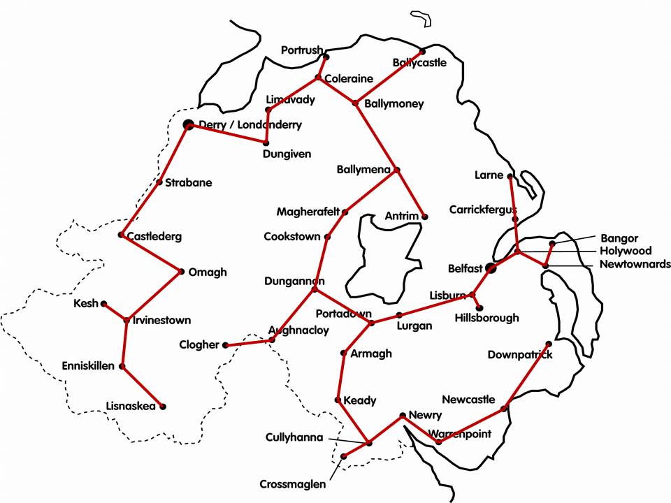
Our MST for the Northern Ireland road network.  What do we make of this then?  Not impressed?  No, that’s not surprising.  Study it for a while to let the full horror sink in …

This is clearly not a realistic design for a road network or infrastructure.  There are all sorts of individual objections but the criticisms will fall broadly into two classes:

1. Vulnerability.  The system is hopelessly susceptible to failure.  An impassible problem, such as an accident or roadworks, between Cookstown and Dungannon, say, completely divides the country in two.  There are no alternative routes, no back-up links.  It won’t be just those two towns that suffer; the whole of the northwest will be cut off from the whole of the southwest.
2. Long routes.  Because there is only ever a single route between any two towns (another essential feature of a tree), some of these routes are very long indeed.  Lisnaskea and Clogher, for example, are geographically close; yet to drive from one to the other involves a trip around half the country.  Similarly, people in Antrim won’t be terribly happy having to drive round the whole of Lough Neagh to reach their near neighbours in Belfast.

Well, of course, we know what a road network generally looks like and it’s not a tree.  In a real road network, we’d expect to see both alternative routes and short routes between close neighbours.  Both of these are usually achieved by building the network in the form of a hierarchy of partial meshes.  A network of local roads connects the entire county but has a further network of major roads overlaid upon it.  At the highest level, motorways connect major cities.  This is what the Northern Ireland road actually looks like (with most of the minor roads left off).

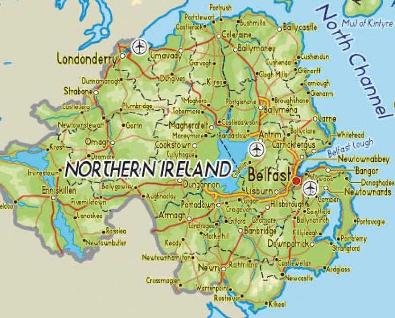
It’s worth noting in passing that most real-world networks – road, rail, water, phone, even the Internet – have really evolved historically rather than ever been optimised as such.  (Evolution, in any context, produces a local optimum rather than a global optimum but that’s another story entirely.)  Here, a typical route from start to finish might involve a local road or two to get to an A road, which in turn leads to a motorway.  The main part of the journey may take place on the motorway, with A roads – then local roads leading to the final destination.  Journeys within local regions will tend to be shorter than those between them and, should there be any problems – blocks or delays, there will always be other ways around.

Now, if were were to try to optimise a network of this form, we’d have two big problems: on one level, the problem becomes very hard to solve; on an entirely different one, it becomes impossible to define in the first place.  This, of course must be explained …

Firstly, once we recognise that we need a network with these alternative routes and multiple levels, we lose the simplicity of the MST problem and the Kruskal and Prim solutions.  It’s just about possible to define a connectivity problem in terms of hierarchical partial meshes but it’s almost impossible to solve.  That is, while the MST is known to be an easy problem in algorithmic terms, whatever problem it’s now become appears to be very hard.  We can’t be sure but it’s unlikely there will be efficient (i.e. quick) algorithms to solve it.  Any attempt at optimisation would only give us a best-effort solution, to which history may have already beaten us.

Secondly, and even more serious, we need to have a much closer look at this idea of ‘cost’, namely the ‘cost’ of each link.  In an abstract graph, costs are just values assigned to each edge.  In a road network, cost depends a bit on the length of an individual road but that’s only part of the story.  Imagine there were no roads at all, i.e. that we’re designing the network from scratch.  What’s the ‘cost’ of the road connecting Antrim to Belfast?

And that, in fact, is an impossible question to answer.  If the road from A to B only carries direct traffic from A to B then we might have a chance.  We’d know it’s length and, more importantly, we’d have an idea of the likely traffic density between the two based on the populations of A and B and the average number of journeys per head of population.  We could dimension the road (local, A-road or motorway) accordingly.  However it’s rarely as simple as that; in practice, the road (A, B) may carry traffic from the other side of A through and beyond B, which may make the road bigger and cost more.  How big (A, B) should be in practice depends on the total traffic it has to carry and this depends on the layout of the rest of the road network.  A genuinely local link will be cheap but an arterial connection expensive.  To dimension – and thus assign a cost to – each potential individual road requires a knowledge of the presence or absence of all the other roads.  The input to our optimisation problem depends on the output.  To describe such a model as ‘poorly formulated’ is something of an understatement.

In fact, now that we see it with this clarity, this would have been an issue with the original MST formulation too.  Assigning costs to the individual links would have been impossible at the outset.  In the solution we arrived at, the road between Cookstown and Dungannon would have carried a huge amount of traffic from most of the northwest to most of the southeast; it would have to be a motorway – and therefore be very expensive – but there was no way of telling this at the start.  We just don’t know what the individual costs are in the manner that we cheerfully assign values to edges in the underlying graph theory.  Yes, MSTs – their formulation and solution – are elegant but, sadly, this just isn’t a valid example of theory being put into practice on any level.

And this uncertainty with regard to cost returns to haunt us if we go back to the earlier example of Internet routing.  Routing protocols, on one level or another, usually work by running some sort of shortest path algorithm to find the preferred route to a destination.  This, in turn, generally involves assigning a ‘cost’ to each individual link indicating the (un)suitability of that link to carry traffic.  (High delay – high cost; High throughput – low cost, etc.)  The commonly used Open Shortest Path First (OSPF) protocol uses Dijkstra’s Shortest Path Algorithm (DSPA) with link costs assigned as the inverse of bandwidth (with the almost obligatory tweak – in this case, of several orders of magnitude).

However, DSPA, in common with most such algorithms only determines shortest paths in isolation – i.e. one route at a time – and that might not work overall.  Choosing high-bandwidth links over smaller ones makes sense only up to the point that we saturate these preferred links by putting too much traffic on them from too many individual routes.  The analogy with the road network works here.  There can be times when the motorways get full and it would be better to divert a fraction of the traffic onto the A roads for the everyone’s benefit.  The cars being diverted aren’t sacrificing themselves for the collective good here – everyone is better off with this improved global solution.  However, the optimal route for each person/car individually is still the motorway (they all have individual sat-navs) so no-one sees the bigger picture.

Trying to look at Internet routing from the wider perspective is problematic for the same two broad reasons as before: complexity and difficulties with defining costs.  However, whilst the transition to a more complex optimisation problem is the same, the ‘cost’ issue is subtly different.  There’s probably some justification in defining simple link costs for routing.  After all, what else could we do?  A high-bandwidth link is a good one and a low-bandwidth one is bad – that can’t be denied.  The problem comes when we try to assign a realistic cost to the overall solution or, more to the point, when we start thinking what exactly it is we’re trying to do.

Solving an optimisation problem involves trying to maximise or minimise some objective function, formed from the values defining a particular instance of the problem.  In the MST case, this is straightforward: “Minimise the total link cost of a connected network from the selected link costs”.  But what about routing?  Minimising costs based on maximising bandwidth is a starting point – not an end in itself.  What are we really trying to maximise or minimise here?  Maximising throughput is nice.  Minimising delay is OK.  Minimising dropped packets is fine.  But these are all bit parts – all different – and none in isolation precisely defines one network from a better one.  Quality of Service sounds good as some sort of compound measure (or see EIGRP’s ‘DUAL’) but what does it actually mean?  What are we ultimately trying to maximise or minimise?  Total number of webpages accessed?  Online purchases?  Customer satisfaction and loyalty?  Company profit?  Worldwide adoption of new technology?  The benefit to humanity?  If anyone can define f in the formula

Global Spiritual Development = f(bandwidth)

then that’s quite an achievement.  This may be taking the point to an extreme but, quite seriously, we don’t actually know what we’re trying to optimise when we run Internet routing protocols; it’s all assumptions that ‘doing X, Y & Z is probably a good thing’.

It’s not easy to round this one off neatly.  It’s certainly untrue to claim that real-world problems can’t be solved or that textbook examples are never used but you have to be really careful.  Just to take the examples we’ve considered:

1. Although costs often can’t be assigned in advance with many network problems, these problems can sometimes be redefined as requirements for network flows.  However, these are always hard to solve and even formulating them is complicated – certainly not a ready example of a real-world application of a simple concept.
2. There’s no doubt that routing algorithms, and related protocols, produce better solutions than simply not bothering.  The doubt is always that we’ve found the best solution – or indeed that we’re even looking for the right thing in the first place.
3. There are applications for spanning trees in the real world – if not exactly minimum spanning trees as we’ve defined.  Certain networking protocols, for example, need to find loop-free ‘backbones’ within complex structures to prevent control packets going around in circles – but these algorithms aren’t trivial.

The difficulty, as always, is matching theory with real-world practice.  There might be some justification in a little simplification for convenience when trying to get a new idea across.  After all, most real-world problems are either too complex for the classroom or have their own shortcuts independent of the textbook.  But when does the convenience of simplification become dishonesty?  Unfortunately, students have a habit of being at their sharpest when we least want them to be!